Visualize posterior distributions or traces from a nested sampling run
Source:R/visualize.R
visualize.ernest_run.RdProduces visualizations of the posterior distributions or the evolution of variables along the log-prior volume from a nested sampling run.
Arguments
- x
[ernest_run] The results of a nested sampling run.
- ...
<
tidy-select> One or more variables to plot from the run. If omitted, all variables are plotted.- .which
[charcacter(1)]Character string specifying the type of plot to produce. Options are"density"for the posterior density of each parameter or"trace"for the trace of variables along log-volume.- .units
[character(1)]
The scale of the sampled points:"original": Points are on the scale of the prior space."unit_cube": Points are on the (0, 1) unit hypercube scale.
- .radial
[logical(1)]
IfTRUE, returns an additional column.radialcontaining the radial coordinate (i.e., the Euclidean norm) for each sampled point.
Value
A ggplot2::ggplot() object.
Details
The visualize() function is designed to quickly explore the results of a
nested sampling run through two types of plots:
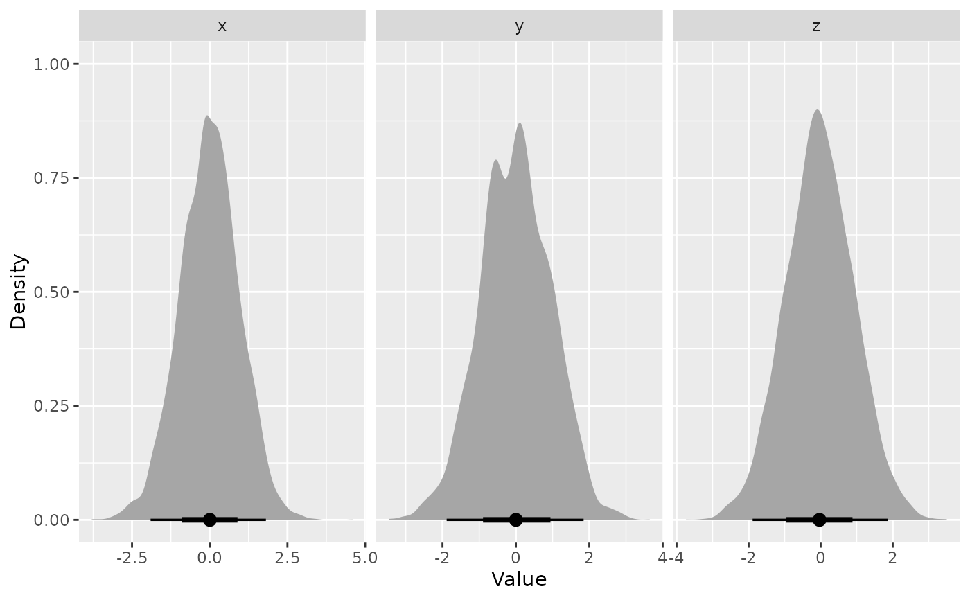
Density plots show the marginal posterior for each selected variable, using
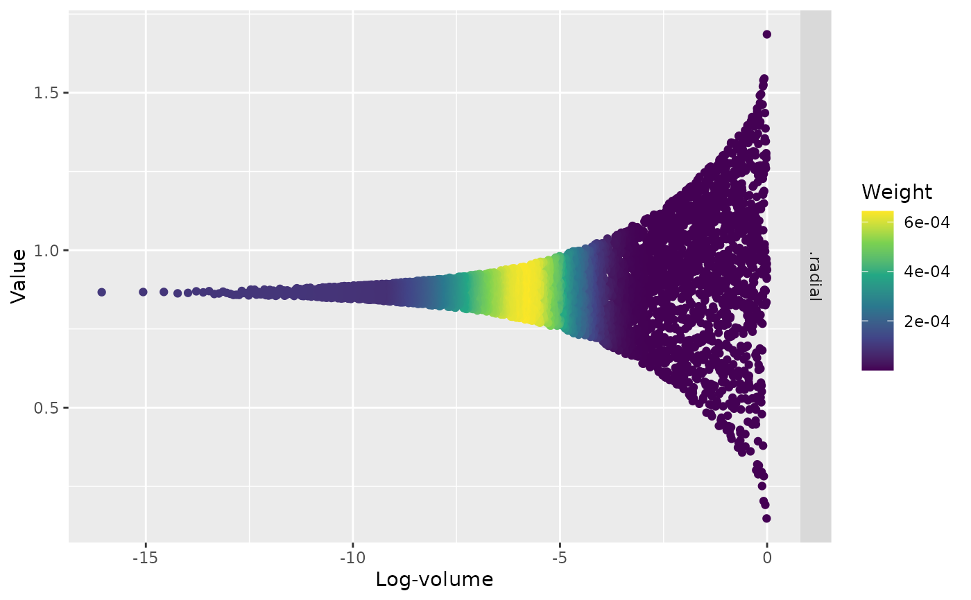
ggdist::stat_halfeye()to visualize uncertainty and distribution shape.Trace plots display the evolution of variables as a function of log-volume, with points coloured by posterior weight. This can help diagnose sampling behavior and identify regions of interest in the prior volume.
Posterior weights are derived from the individual contributions of each sampled point in the prior space to a run's log-evidence estimate. A point's weight is a function of (a) the point's likelihood and (b) the estimated amount of volume within that point's likelihood contour. See ernest's vignettes for more information.
Note
This package requires the tidyselect package to be installed. If
which = "trace" is selected, the ggdist package is also required.
See also
plot()for diagnostic plots of nested sampling runs.as_draws_rvars()for extracting posterior samples.