Transform nested sampling runs to draws objects

Convert an ernest_run to a format supported by the posterior package.

Usage

# S3 method for class 'ernest_run'
as_draws(x, ..., units = c("original", "unit_cube"), radial = FALSE)

# S3 method for class 'ernest_run'
as_draws_matrix(x, ..., units = c("original", "unit_cube"), radial = FALSE)

# S3 method for class 'ernest_run'
as_draws_rvars(x, ..., units = c("original", "unit_cube"), radial = FALSE)

Arguments

x

An ernest_run object.

...

These dots are for future extensions and must be empty.

units

Case-sensitive string. The scale for the sampled points:

• "original": Points are on the scale of the prior space.

• "unit_cube": Points are on the (0, 1) unit hypercube scale.

radial

Logical. If TRUE, returns an additional column .radial containing the radial coordinate (i.e., the Euclidean norm) for each sampled point.

Value

A draws object containing posterior samples from the nested sampling run, with importance weights (in log units).

The returned object type depends on the function used:

• For as_draws and as_draws_matrix, a posterior::draws_matrix() object (class c("draws_matrix", "draws", "matrix")).

• For as_draws_rvars, a posterior::draws_rvars() object (class c("draws_rvars", "draws", "list")).

See also

• posterior::as_draws() for details on the draws object.

• posterior::resample_draws() uses the log weights from ernest's output to produce a weighted posterior sample.

Examples

# Load example run
library(posterior)
#> This is posterior version 1.6.1
#> 
#> Attaching package: ‘posterior’
#> The following objects are masked from ‘package:stats’:
#> 
#>     mad, sd, var
#> The following objects are masked from ‘package:base’:
#> 
#>     %in%, match
data(example_run)

# View importance weights
dm <- as_draws(example_run)
weights(dm) |> head()
#> [1] 9.246773e-63 3.843403e-62 8.700225e-60 2.020381e-58 1.866047e-55
#> [6] 1.975416e-54

# Summarise points after resampling
dm |>
  resample_draws() |>
  summarize_draws()
#> # A tibble: 3 × 10
#>   variable     mean   median    sd   mad    q5   q95  rhat ess_bulk ess_tail
#>   <chr>       <dbl>    <dbl> <dbl> <dbl> <dbl> <dbl> <dbl>    <dbl>    <dbl>
#> 1 x         0.00624  0.0225  0.946 0.931 -1.58  1.54  1.17    2103.     14.7
#> 2 y        -0.00852 -0.00513 0.975 0.989 -1.60  1.57  1.17    1916.     14.5
#> 3 z        -0.0256  -0.0295  0.963 0.952 -1.60  1.56  1.17    2124.     14.2

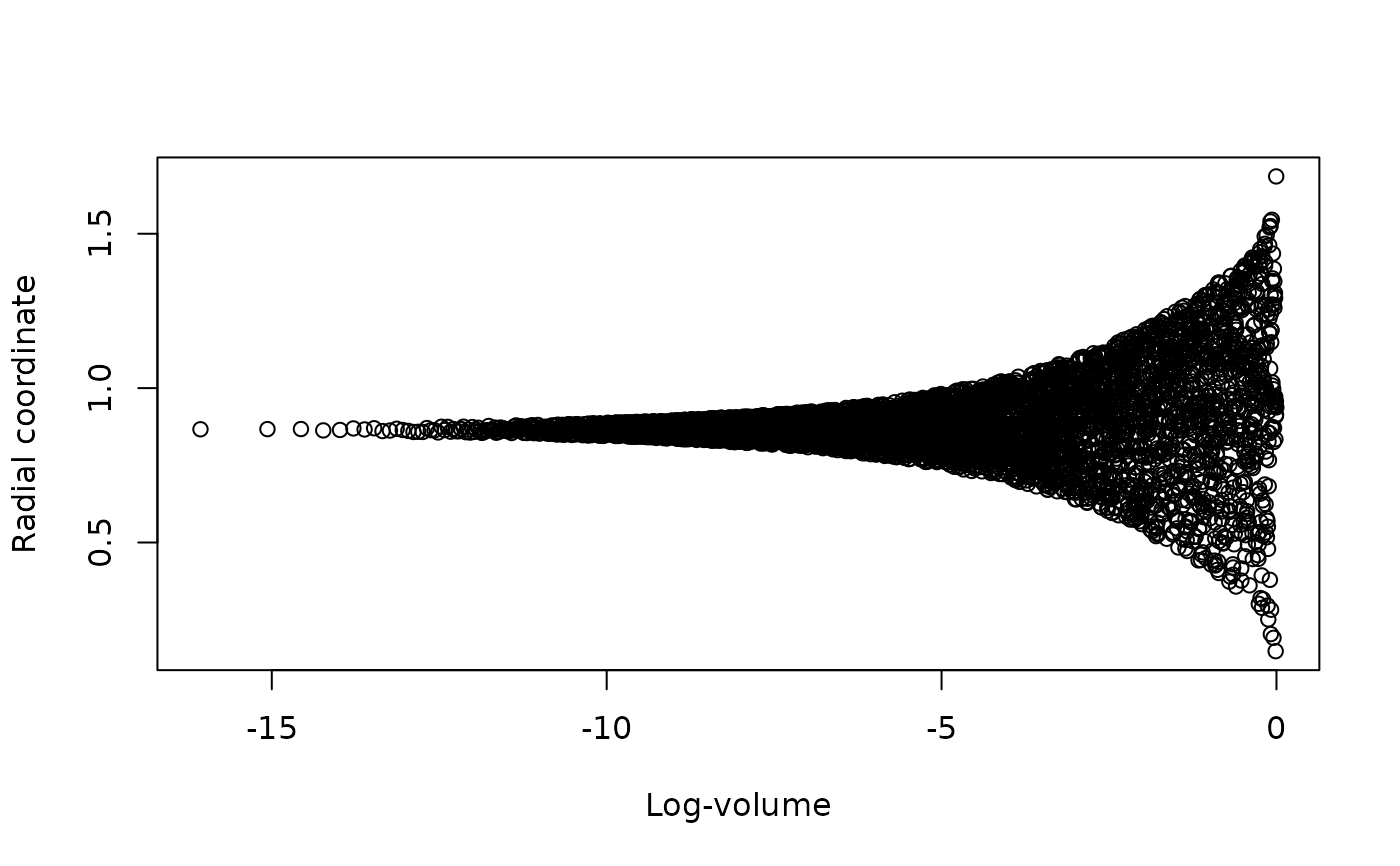
# View the radial coordinate in unit space over the run
dm_rad <- as_draws_rvars(
  example_run,
  units = "unit_cube",
  radial = TRUE
)
plot(
  x = example_run$log_volume,
  y = draws_of(dm_rad$.radial),
  xlab = "Log-volume",
  ylab = "Radial coordinate"
)