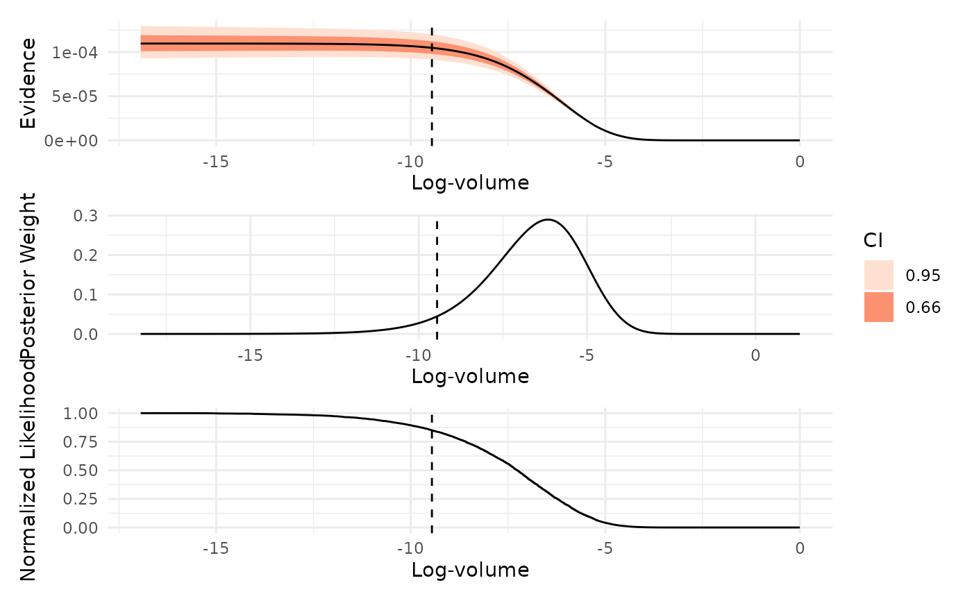
Plot diagnostics for a nested sampling run

Visualizes key diagnostics from a nested sampling run, including the normalized likelihood, posterior weights, and evidence as functions of log-prior volume.

Usage

# S3 method for class 'ernest_estimate'
plot(x, which = c("evidence", "weight", "likelihood"), ...)

# S3 method for class 'ernest_run'
plot(x, which = c("evidence", "weight", "likelihood"), ndraws = NULL, ...)

Arguments

x: [ernest_run] or [ernest_estimate]
An object containing results from nested sampling.
which: [character()]
Choose which plots to display. Must be one or more of "evidence", "weight", and "likelihood".
...: These dots are for future extensions and must be empty.
ndraws: [integer(1)]
The number of log-volume sequences to simulate. If equal to zero, no simulations will be made, and a one draw vector of log-volumes are produced from the estimates contained in x.

Value

[invisible(x)]. A ggplot2::ggplot() object is printed as a side effect.

Details

Interpreting these plots can help diagnose issues such as poor or insufficient prior sampling and model misspecification. Use which to select the plots to display:

which = "evidence": Plots the estimated marginal likelihood (evidence) as a function of log-prior volume, with uncertainty intervals. Peaks in this plot indicate regions of prior volume that contribute most to the evidence estimate.
which = "weight": Shows the distribution of posterior mass across log-prior volume. This plot highlights which regions of the prior volume contain the most posterior probability, helping to identify where the sampler concentrated its effort.
which = "likelihood": Displays the normalized likelihood as a function of log-prior volume. Smoothness in this plot indicates effective likelihood-restricted prior sampling, while irregularities may suggest sampling difficulties or, in some cases, misspecified likelihood functions.

If x is an ernest_run, the plots are based on the actual run data. Error ribbons are drawn around the evidence plot from analytic estimates of uncertainty (see summary.ernest_run).

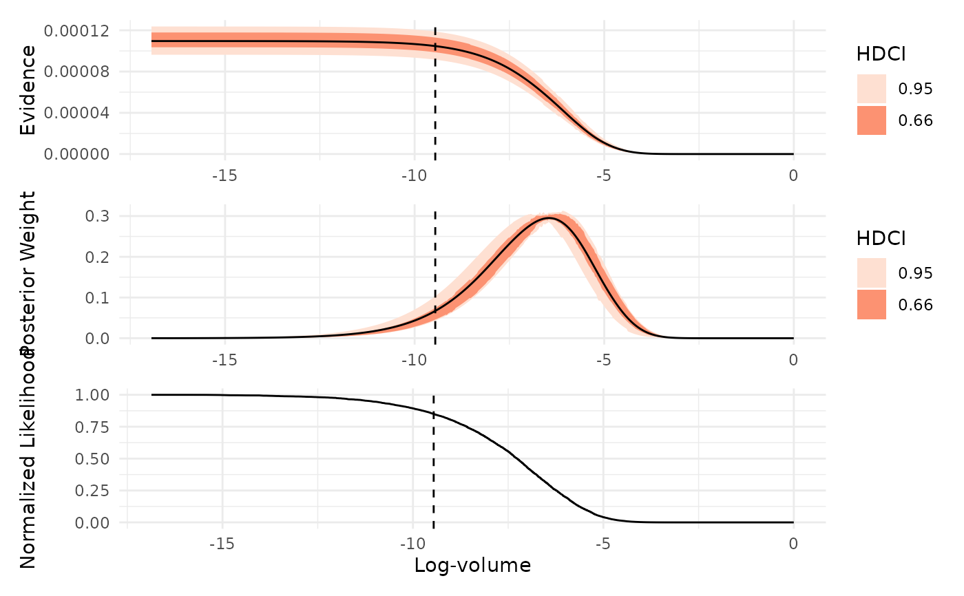
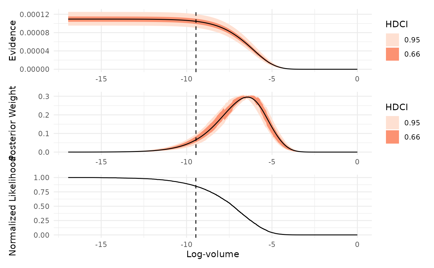
If x is an ernest_estimate (or if ndraws is specified), the plots are based on simulated values from the log-volume. The highest density continuous intervals (HDCIs) are computed using ggdist::median_hdci() for both the evidence and weight plots.

Note

Plotting multiple diagnostics with which requires the patchwork package. Plotting ernest_estimate objects requires the ggdist package.

Examples

# Plot results from a run.
data(example_run)
plot(example_run)


# Simulate results before plotting.
set.seed(42)
plot(example_run, ndraws = 100)


# Equivalently, simulate results, then plot:
set.seed(123)
est <- calculate(example_run, ndraws = 100)
plot(est)