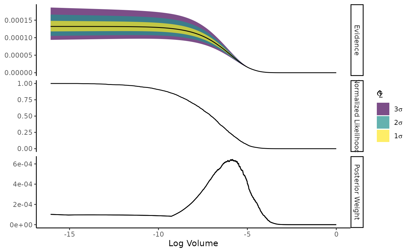
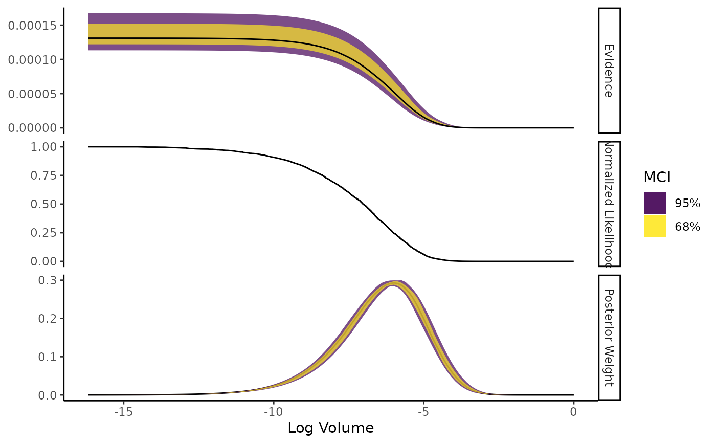
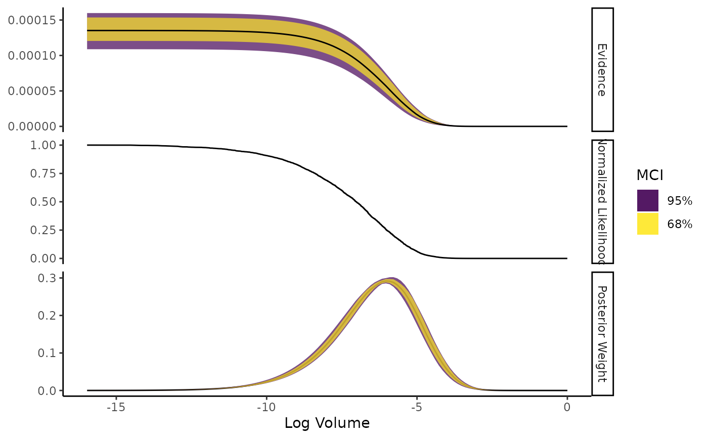
Shows the normalised likelihood, importance weights, and evidence as functions of log-volume.
Arguments
- x
An ernest_estimate or ernest_run object.
- ...
These dots are for future extensions and must be empty.
- ndraws
An optional positive integer. The number of log-volume sequences to simulate. If equal to zero, no simulations will be made, and a one draw vector of log-volumes are produced from the estimates contained in
x. IfNULL,getOption("posterior.rvar_ndraws")is used (default 4000).
Value
Invisibly returns x. A ggplot2::ggplot() object is printed as a
side effect.
The plot is faceted into three panels. The horizontal axis shows log-volume:
If x is an ernest_run, these estimates are derived from the run;
if x is an ernest_estimate (or ndraws != 0), these values are
simulated.
The three y axes are:
Evidence: Estimate with an error ribbon drawn from either the estimated standard error (if
ernest_run) or from the median credible interval (MCI) (ifernest_estimate);Normalised Likelihood: The likelihood value of the criteria used to draw new points from the likelihood-restricted prior sampler, normalised by the maximum likelihood generated during the run;
Posterior Weight: The density of the posterior weights attributed to regions of volume within the prior. For
ernest_estimateobjects, an error ribbon is drawn with the MCI of this estimate.
See also
calculate()for generatingernest_estimateobjects.visualize()for plotting the posterior distributions generated by a run.