Access the posterior sample and weights from a nested sampling run as an object supported by the posterior package.
Usage
# S3 method for class 'ernest_run'
as_draws(x, units = c("original", "unit_cube"), radial = FALSE, ...)

# S3 method for class 'ernest_run'
as_draws_matrix(x, units = c("original", "unit_cube"), radial = FALSE, ...)

# S3 method for class 'ernest_run'
as_draws_rvars(x, units = c("original", "unit_cube"), radial = FALSE, ...)
Arguments
- x
[ernest_run]
Results from a nested sampling run.- units
[character(1)]
The scale of the sampled points:"original": Points are on the scale of the prior space."unit_cube": Points are on the (0, 1) unit hypercube scale.
- radial
[logical(1)]
IfTRUE, returns an additional column.radialcontaining the radial coordinate (i.e., the Euclidean norm) for each sampled point.- ...
These dots are for future extensions and must be empty.
Value
posterior::draws_matrix() or posterior::draws_rvars()
A object containing the posterior samples from the nested sampling run,
with a hidden .weights column containing the importance weights for each
sample.
Note
To produce a weighted posterior sample, use
posterior::resample_draws() to reweigh an object from as_draws using its
importance weights.
See also
posterior::as_draws()for details on thedrawsobject.
Examples
library(posterior)
#> This is posterior version 1.6.1
#>
#> Attaching package: ‘posterior’
#> The following objects are masked from ‘package:stats’:
#>
#> mad, sd, var
#> The following objects are masked from ‘package:base’:
#>
#> %in%, match
data(example_run)
# View importance weights
dm <- as_draws(example_run)
weights(dm) |> head()
#> [1] 1.319439e-63 5.734565e-61 6.105971e-59 1.221066e-58 8.797702e-58
#> [6] 2.620611e-56
# Summarise points after resampling
dm |>
resample_draws() |>
summarize_draws()
#> # A tibble: 3 × 10
#> variable mean median sd mad q5 q95 rhat ess_bulk ess_tail
#> <chr> <dbl> <dbl> <dbl> <dbl> <dbl> <dbl> <dbl> <dbl> <dbl>
#> 1 x -0.0254 -0.0388 0.964 0.952 -1.63 1.55 1.19 4202. 13.0
#> 2 y 0.00483 0.00671 0.980 0.974 -1.60 1.60 1.19 4455. 12.6
#> 3 z 0.0129 0.0320 0.987 0.968 -1.62 1.63 1.19 4113. 12.5
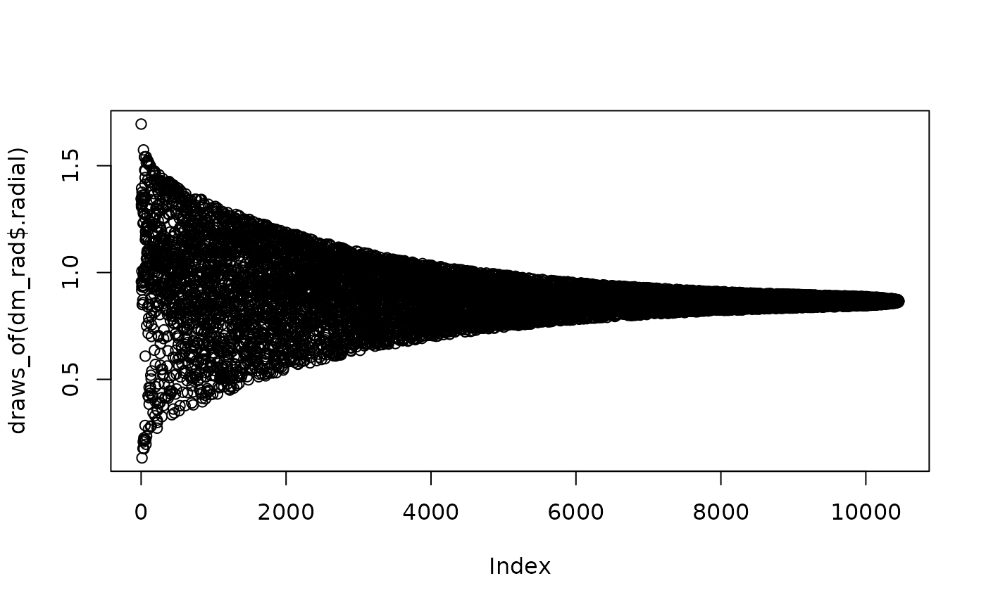
# View the radial coordinate in unit space over the run
dm_rad <- as_draws_rvars(
example_run,
units = "unit_cube",
radial = TRUE
)
plot(x = draws_of(dm_rad$.radial))